Mean-Variance Frontier

Mean-variance optimization is one of those topics that has always been awkward to teach with spreadsheets. It is messy to define the portfolio variance in a spreadsheet for more than two assets, and we are forced to use Solver to find efficient portfolios or to deal with Excel’s matrix algebra functions that operate on arrays. Also, if we create an example for three assets and someone asks about four, then we have to almost entirely reengineer the spreadsheet. I don’t think we actually expect students to do mean-variance analysis in a spreadsheet after they graduate - we’re just teaching the concept (I think). But, we can now teach the concept without the clunkiness of setting it up in a spreadsheet.
We want to generate the classic figure above and to find the portfolios crresponding to the efficient mean-variance combinations. I prefer to start with the tangency portfolio, because it is simpler than finding the frontier of only risky assets, and because it is where we want to end up anyway. We can specify the risk-free rate, the expected returns of the assets, the standard deviations of the assets and their correlations and just ask Julius to compute the tangency portfolio. The LLMs know how to do it. With high probability, they will generate code to compute the familiar Sigma inverse times mu and then divide by the sum of the elements of that vector so the weights sum to one (it is possible but much less likely that they will use a numerical optimization algorithm from scipy to maximize the Sharpe ratio). This means that we have to explain Sigma inverse times mu.
I take a very hand-waving approach to explain the formula. I remind students first that at the top of a hill the slope must be zero and second that the slope of a function is its derivative, so a maximum is the solution of an equation “derivative = 0.” Of course, they have all seen that at some point in their lives. I then show them (without deriving) the equations for maximizing the Sharpe ratio with three risky assets:
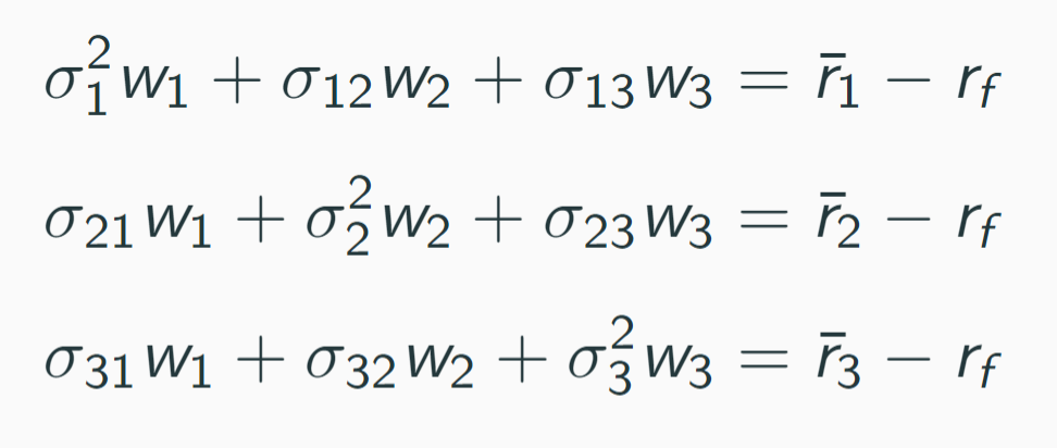
I explain that this system of equations is written as Sigma times w equals risk premia, explaining matrix multiplication briefly, and then say that it can be solved for w with a matrix version of “dividing by” Sigma. That seems to give enough intuition for the formula w = Sigma inverse times risk premia.
Asking next for the global minimum variance portfolio is a natural thing to do. The LLM is likely to use the calculus/algebra solution for that also. It is of course the same process as calculating the tangency portfolio but with the risk premia replaced by a vector of constants, for example, a vector of 1’s. If we then ask for the portfolio of only risky assets that achieves a target expected return with minimum risk, we are more likely to see the LLM use an optimizer from scipy. Here, too, I have seen Claude use the calculus/algebra solution, but it is a bit more complicated and evidently appeared less often in the training data than did the solution for the tangency portfolio.
We can also impose position limits, including short sales constraints. In fact, the “no short sales” constraint seems to have appeared so often in the training data that the LLM may impose it when it uses an optimizer even if you have not asked for it. It pays to check the code. If students look, they should be able to decipher the code well enough to see if nonnegativity constraints were imposed. It is also pretty reliable to just ask the LLM if it used nonnegativity constraints, or you may want to say explicitly not to impose them if you don’t want them (to get it to obey, you may need to be emphatic: “It is important that you do not impose short sales constraints. Please pay attention to this.”)
Mean-variance optimization is used in practice mainly for strategic asset allocation, so it is good to demonstrate it on asset classes. Yahoo ETF data is an easy source, though the time series is short. Aswath Damodoran maintains some data on his website at NYU, in particular this. If students want to check their results, they could do so with this page and this from the website I created with Kevin Crotty. I’ve always liked the Harvard Management Company case from HBS for teaching mean-variance analysis, because it provides some perspective on the unreliability of unconstrained mean-variance optimization (and the fact that imposing position constraints may mean that you just get your constraints back as the solution).
Please share your thoughts in the comments below.
Also on substack at kerryback.substack.com